Every Infinity Paradox Explained

Thanks for watching 🙂

Watch Next:

Playlists:

Timestamps:

0:00 Hilbert’s Hotel
1:07 Cantor’s Diagonal Argument
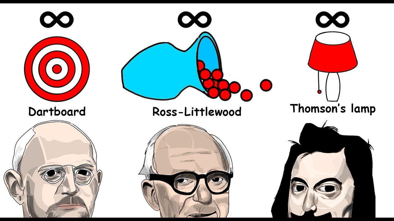
3:22 Thomson’s Lamp
5:16 Gabriel’s Horn
7:23 Ross-Littlewood Paradox
8:51 Dartboard Paradox
10:47 Sponsor
11:50 St. Petersburg Paradox
13:18 Riemann Series Theorem

— DISCLAIMER —

This video is intended for entertainment and educational purposes only.

Hilbert’s Hotel

Hilbert’s Hotel is a thought experiment proposed by German mathematician David Hilbert in 1925. It involves a hotel with an infinite sequence of rooms: 1, 2, 3, and so on to infinity. This is called countable infinity, since each room can be associated with a counting number. The hotel starts out fully occupied.

However, a new person shows up and wants a room. Surprisingly, you can accommodate the new guest without removing any current guests. The hotel simply moves the guest in Room 1 to Room 2, the one in Room 2 to Room 3, and so on. In general, the guest in room n moves to room n + 1. Afterward, Room 1 is free for the new guest.

Hilbert’s Hotel can also accept a countably infinite number of new guests. The guest in Room 1 moves to Room 2, the one in Room 2 to Room 4, and in general the guest in room n moves to room 2n. This leaves the odd-numbered rooms free for the new guests.

The fact that Hilbert’s Hotel can accommodate new guests despite being full is known as Hilbert’s Paradox. This is an example of a veridical paradox, a statement that is true despite seeming false.

Cantor’s Diagonal Argument

Cantor’s diagonal argument is a proof that the cardinality of the set of real numbers is greater than the cardinality of the set of natural numbers. The cardinality of a set can be thought of as its size. This proof was published by Georg Cantor in 1891.

To prove this fact, it is sufficient to show that there are more real numbers between 0 and 1 than there are natural numbers. If this is the case, then there are definitely more real numbers than natural numbers.

The proof is by contradiction. A proof by contradiction starts with an assumption and shows that the assumption leads to an impossible conclusion, thus proving that the assumption is wrong. In Cantor’s diagonal argument, we begin by assuming that the set of real numbers between 0 and 1 and the set of natural numbers have the same cardinality. If so, that means each real number can be paired with a natural number one-to-one with no numbers left over.

So let’s do that and put the pairs in a list. Our list of pairs will have the natural numbers on the left and the real numbers on the right, making sure the digits of the real numbers are aligned with each other. Then we draw a downward-right diagonal through the digits of the real numbers.

Now let’s construct a new real number. Starting at the top left of the diagonal, take the first digit of the first real number and change it to something else. For example, if it is 9, subtract 1 from it; otherwise, add 1. Put this digit in our new number. Now go down the diagonal, repeating this process for all the real numbers in the list.

Is our new number part of the list? It can’t be the first number in the list, since the first digits don’t match. It can’t be the second number either, since the second digits don’t match. Our new number will always differ from any given number in the list, since there will always be at least one digit that does not match the digit on the diagonal. Thus we have a real number that isn’t part of the list, meaning we haven’t achieved a one-to-one pairing, which contradicts our earlier assumption. Even if we insert this new number into the list, we can just repeat this process to generate more and more new real numbers. This implies that there are more real numbers than there are natural numbers.

The idea that some infinities are bigger than others is counterintuitive, but it is a true fact.

Thompson’s Lamp

Thompson’s lamp is a hypothetical device proposed by British philosopher James F. Thomson in 1954. It is a lamp that can be switched on and off as fast as you want. Let’s say that you start a timer and turn the lamp on. You wait 1 minute and then you turn the lamp off. After another half minute has passed, you turn the lamp back on. Each time, you wait for half of the previous amount of time and then toggle the lamp.

Because the lengths of these intervals add up to 2 minutes, you will have toggled the lamp an infinite number of times after 2 minutes have passed. A task like this, with an infinite amount of action in a finite amount of time, is called a supertask. But when you are finished, will the lamp be on or off? Each time you toggle the lamp off, it was immediately followed by toggling it back on, and vice versa. Thus it seems like the question has no logical answer, which creates a paradox.

Mathematically, this is related to the behavior of the infinite sum 1 − 1 + 1 − 1 and so on forever. An infinite sum like this is called a series, and this particular one is called Grandi’s series, named after Italian mathematician Guido Grandi. Because the result just bounces back and forth between 0 and 1 forever as you take more and more terms, the series doesn’t approach a specific number (or converge), so we say that it diverges or has no finite value.

However, certain methods can be used to assign the series a meaningful value. For instance, you can take the averages of the partial sums as you go along, known as the Cesàro method, which gives a value of 1/2. Thomson had heard of Grandi’s series being given this value, but his thought experiment did not allow the possibility of the lamp being “half on.” Thus he rejected that Grandi’s series and his thought experiment had any direct relation.

Gabriel’s Horn

Gabriel’s horn is an infinitely long horn-shaped object with a finite volume but an infinite surface area. It was first considered by Italian mathematician Evangelista Torricelli in a paper published in 1643.

In order to form Gabriel’s horn, take the graph of the curve y = 1/x in the xy-plane with the domain x ≥ 1. Then rotate this curve in three dimensions around the x-axis, forming a surface of revolution. Now imagine closing off Gabriel’s horn with a cap. We can find the volume of the inside region using integration.

Using slices perpendicular to the x-axis, slice the inside region into thin discs that are approximately thin cylinders. Labeling the radius of each cylinder as r, the base area of each cylinder is πr², and the little thickness is dx. So the volume is approximately πr² · dx. The radius at each point is just the distance between the x-axis and the graph of the function 1/x, so we can replace r with 1/x. The volume of each cylinder is approximately π · (1/x²) · dx, and we just have to integrate this from 1 to ∞, which gives us π. So the volume of this region is π.

But what about the area under the curve y = 1/x from 1 to ∞? As the upper bound grows bigger and bigger, the natural logarithm of that bound also grows without limit. So the area under the curve is actually infinite, despite the fact that when we rotate this curve around the x-axis, the volume of the resulting solid has a finite value of π. Due to the counterintuitiveness of this fact, mathematicians at the time of its discovery perceived it as a paradox.

The Ross-Littlewood Paradox

The Ross-Littlewood Paradox, invented by John E. Littlewood in 1953 and further explored by Sheldon Ross in 1988, involves an infinitely large empty vase and an infinite number of balls. A supertask is performed: at each step, 10 balls are put in the vase and then one ball is taken out. Each step takes half the amount of time as the previous one, to ensure that the task is completed in a finite amount of time.

Now, at the end, how many balls does the vase contain? The intuitive answer appears to be infinitely many. Each step seems to involve a net increase of 9 balls in the vase, so the number of balls just grows toward infinity.

However, there is a sense in which the vase may be empty. Imagine that at the start, all of the balls are numbered. At step one, you put in balls 1 through 10 and remove ball 1. At step two, you put in balls 11 through 20 and remove ball 2. And so on. For each step number n, the ball numbered n is removed from the vase. Eventually ball number 1,000 will be removed, then ball number 1,000,000, and so on. Since there are no balls that don’t eventually get removed, by the end all of the balls must have come out.

There is no general agreement on the solution to this paradox. Besides the previous solutions, some people think it depends on exactly which balls you take out of the vase. Others think that the problem does not give us enough information to state the answer, or that it isn’t well defined.

The Dartboard Paradox

The dartboard paradox is a paradox in probability. Let’s say you have a dartboard and you randomly pick some point on it. Now a dart hits the dartboard at a random point. Is it possible for the dart to exactly hit the point you picked? And if so, what is the probability that this occurs? This is a mathematical scenario, so we will assume that the point is infinitely small.

The answer to the first question is obviously yes, since the dart can hit any point on the dartboard. However, since your point is only one point out of infinitely many, it seems that the probability of hitting that point is actually zero. Indeed, in a rigorous mathematical sense, this is actually the case. But you can use the same logic for any other point on the dartboard. So the probability of the dart hitting any given point on the dartboard is zero as well.

This seems counterintuitive, since we said that a dart must hit the dartboard. The problem is that probability zero does not mean impossible. What we have here is known as a continuous random variable, because the space of possible contact points for the dart is continuous. This is as opposed to a discrete random variable, where there are only a finite number of possible outcomes, such as the roll of a die.

Continuous random variables are common in probability. For example, the normal distribution models a continuous random variable. In this case, it is often more useful to talk about the probability that a given event falls within a specific region of the possibilities. For example, you can ask about the probability that the dart will land on the dartboard’s upper right quadrant. In this case, the probability is 1/4, or 25%. When using a continuous distribution such as the normal distribution, the probability of an event happening in a certain region is equal to the area between the graph of the distribution and the horizontal axis within that region, which can be calculated using integration.

The St. Petersburg Paradox

The St. Petersburg Paradox is another probability-based paradox, named for the city where Daniel Bernoulli studied it. Imagine a casino game beginning with a stake of $2. The stake is the amount the player will be paid at the end. The player flips a coin, and if it lands on tails, the stake doubles. Otherwise, the game ends and the player gets the stake.

We can calculate the expected value of the player’s earnings. The expected value is the average value that you would predict from a random process. There is a 1/2 chance that the player lands on heads immediately, earning $2. Given the 1/2 chance of landing on tails to start with, there is then a 1/2 chance of landing on heads on the next flip and earning $4, giving an overall chance of 1/4 to earn $4. This logic continues for all remaining flips.

We can calculate the expected value by multiplying each payout by its probability and adding the results together: 1/2 × 2 + 1/4 × 4 + 1/8 × 8 + … is the same as 1 + 1 + 1 + …, which goes to infinity.

Now what would be a fair cost to play this game? Hypothetically, no matter the cost, even if it were $1 billion, the casino always loses. However, according to Ian Hacking, few people would pay even $25 to play this game, which is the paradox.

The Riemann Series Theorem

The Riemann series theorem, named for and rigorously proved by German mathematician Bernhard Riemann, involves conditionally convergent series. A conditionally convergent series is an infinite sum that converges to a particular finite value but would not converge if you added up the absolute values of the terms instead. In other words, a conditionally convergent series converges only under the condition that the sign of each term is taken into account. This is as opposed to an absolutely convergent series, which converges in both cases.

According to the Riemann series theorem, any given conditionally convergent series can be rearranged to produce any real number. This runs counter to how finite sums work, where rearrangement of the terms doesn’t affect the result.

To prove the Riemann series theorem, consider grouping all the terms of a conditionally convergent series into two groups, positive and negative, in descending order of magnitude. Since the series is convergent, the magnitudes of the terms in each group must get arbitrarily small. However, remember that the series is only conditionally convergent. That means each group of terms individually doesn’t sum to a finite value. If the positive terms were to sum to some positive value a and the negative terms to some negative value −b, then the overall sum of the absolute values would be a + b, implying that the series would be absolutely convergent, not conditionally convergent.

It’s also impossible that the positive terms sum to positive infinity while the negative terms sum to a finite negative value, because the original series would then diverge toward positive infinity, not converge. The same logic applies in reverse. Thus the only possibility is that the positive terms sum to positive infinity and the negative terms sum to negative infinity.

Due to the fact that these are unbounded, we can combine terms to reach any target. To test this, pick any real number x and try to get to it by adding terms. Start at zero. If x is above where you are, add the largest positive term you haven’t used. If x is below, add the negative term of greatest magnitude that you haven’t used. If you’re currently at x, you can add either. Repeating this process indefinitely, going as far up or down as needed, you gradually converge on x as the terms get smaller and smaller.

This article was generated from the video transcript of “Every Infinity Paradox Explained”.
Watch the full video above for visual explanations and diagrams.