Simpson’s Paradox
Simpson’s Paradox is often presented as a compelling demonstration of why we need statistics education in our schools. It was first noted by Edward H. Simpson in 1951, who observed that overall combined data can sometimes mask important insights that become evident when looking at subgroups. This paradox occurs when trends observed in different groups of data reverse upon combining those groups.
Assume that there is a new treatment for a disease. You look at two groups, both males and females. Among males, 70% of treated patients survive while only 30% of untreated patients survive. Among females, 80% of treated patients survive while only 40% of untreated patients survive. Based on these separate groups, it seems like the treatment is very effective for both males and females.
Now let’s combine the data. In the combined group of males and females, 50% of treated patients survive while 60% of untreated patients survive. Surprisingly, when you look at the combined data, it appears that the treatment is less effective or even harmful. This reversal of the trend when the groups are combined is known as Simpson’s Paradox.
The paradox happens because of a third variable called a confounder, which affects the two groups differently. In this case, the third variable could be something like the severity of the disease, which might vary between males and females, affecting the overall survival rates. To decide whether the treatment is truly effective, you need to look at the data carefully, considering the impact of the third variable. In some cases the combined data gives the right conclusion, and in others the separate groups give the correct answer.
The Monty Hall Problem
You’re on a game show and there are three doors. Behind one door is your dream car, and behind the other two are goats. You pick a door, let’s say Door A. Then the host, Monty Hall, who knows exactly what’s behind each door, opens another door, say Door B, revealing a goat. Now he gives you a choice: stick with your original choice, Door A, or switch to the remaining unopened door, Door C.
Intuitively it might seem like it doesn’t matter if you switch or not, because there are two doors left, so the chances should be 50/50. But surprisingly, if you switch doors you actually have a higher chance of 2/3 of winning the car, compared to your initial choice of 1/3.
The key insight is that Monty’s action of revealing a goat provides new information that changes the underlying probabilities. Initially each door has a 1/3 chance of hiding the car. After Monty opens a door with a goat, the door you initially picked still has a 1/3 chance, but the combined probability for the other two doors, since Monty won’t reveal the car, becomes 2/3. Therefore, switching to the other door increases your chances of winning to 2/3.
Now scale it up. If there are 100 doors, behind one is a new game console and behind the others are goats. You pick Door 1. Monty opens 98 other doors, all goats. Now you have Door 1 and Door 73 left. Should you stick or switch? Switching to Door 73 now gives you a 99% chance of winning, because Monty’s actions show where the goats are, making Door 73 very likely to have the console.
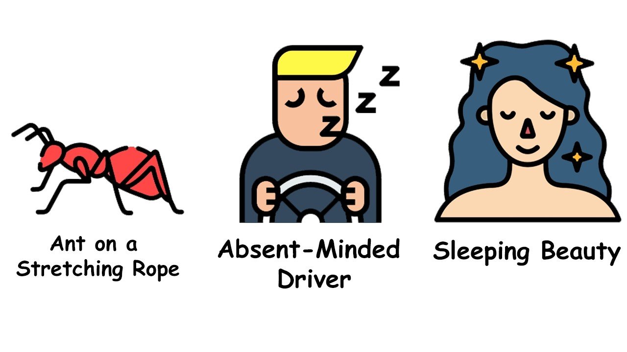
The Sleeping Beauty Problem
Sleeping Beauty agrees to participate in an experiment. On Sunday she is given a sleeping pill and falls asleep. During the experiment a coin is tossed secretly. If it lands on heads, she’s woken up on Monday, given another sleeping pill, and then woken up again on Wednesday. If it lands on tails, she’s woken up on both Monday and Tuesday, each time given a sleeping pill, and then woken up again on Wednesday. Each time she wakes up, she doesn’t know if it is Monday or Tuesday, and she doesn’t know the outcome of the coin toss.
Put yourself in the position of Sleeping Beauty. You wake up. You don’t know what day it is and you don’t know if you have been woken up before. You only know the theoretical course of the experiment. The question: what is the probability that the coin landed heads when she is asked about it after each waking?
One camp argues it should be 1/2 (50%), because at the start of the experiment, whether it’s heads or tails is equally likely regardless of the day she wakes up. The other camp argues it should be 1/3 (about 33.3%), because there are three scenarios: heads on Monday, tails on Monday, and tails on Tuesday. Since tail scenarios happen twice as often as head scenarios (once for Monday and once for Tuesday), the probability should be 1/3.
Imagine repeating the experiment many times. In the long run, Sleeping Beauty would wake up after heads roughly 1/3 of the time and after tails on Monday or Tuesday each roughly 1/3 of the time, for a 2/3 total for tails. This long-run reasoning should apply to the single trial as well, suggesting 1/3 for heads.
The Sleeping Beauty problem is a famous thought experiment with no universally agreed-upon answer.
Cantor’s Paradox
Imagine you have a set A that contains smaller subsets. These subsets could be any groups within A, like different categories of animals in a zoo or types of books in a library. Cantor showed that the number of these subsets, let’s call it P(A), the power set of A, is always greater than the number of elements in A itself. This means if A has, say, three elements, its power set P(A) will have more than three subsets. This discovery was surprising because intuitively we might think that the whole set A should have the most things since it contains everything. But Cantor demonstrated that in terms of cardinality, the collection of subsets can be larger.
In mathematical terms, Cantor’s theorem states that for any set A, the cardinality (which measures the size or number of elements) of its power set P(A) is strictly greater than the cardinality of A itself. Formally, if |A| denotes the cardinality of A, then |A| < |P(A)|.
Here’s why this is true. The power set P(A) is the set of all subsets of A. To show that |A| < |P(A)|, Cantor used a diagonal argument, which proves that there cannot be a bijection (a one-to-one correspondence) between A and P(A). In simpler terms, even though A might have a certain number of elements, its power set P(A) includes every possible way to group these elements into subsets. This results in P(A) having more subsets than there are individual elements in A.
This mathematical insight was groundbreaking because it revealed that there are different levels or sizes of infinity, challenging our intuitive understanding of size and countability in mathematics.
The Ant on a Stretching Rope
Imagine an ant standing at one end of a rubber rope that’s initially 1 km long. The ant crawls at a steady pace of 1 cm per second. However, every second the rope stretches uniformly. After the first second it’s 2 km long, after the second second it’s 3 km long, and so on. The question is whether the ant will ever reach the far end of this rope.
Surprisingly, the answer is yes. Initially the ant moves forward 1 cm, which is 1/100,000th of the original 1 km length. After the first second, when the rope stretches to 2 km, the ant moves another centimeter, and now that centimeter is 1/200,000th of the new 2 km length. If you sum up all these fractions over time, it forms a series. This series is known as the harmonic series, and it actually diverges to infinity. This means that no matter how large the rope stretches each second, the sum of these fractions will eventually exceed one, ensuring that the ant will reach the end of the rope.
Berry’s Paradox
Berry’s Paradox is about how we define numbers with very specific rules. Imagine trying to define a number using a description that states it cannot be described in fewer than 23 syllables. The catch is that the phrase itself has only 20 syllables. This creates a contradiction, because the number it defines supposedly requires more syllables to describe than the phrase itself.
Berry’s Paradox extends beyond mere wordplay. It has implications in fields like algorithmic information theory. Specifically, it suggests limits on the ability to compute the Kolmogorov complexity of a string. Kolmogorov complexity measures the shortest computer program or description that can produce a given string. But Berry’s Paradox hints at cases where such descriptions might become self-contradictory or impossible to construct. It highlights deeper issues in defining and computing complex entities based on their descriptions or definitions.
The Absent-Minded Driver
An absent-minded driver starts at a point called Start on a map. From there they encounter an intersection called X. At X, the driver can either exit and end up at location A with a payoff of zero, or they can continue to another intersection called Y. At Y, the driver faces another decision: exit to get to location B with a payoff of four, or continue to location C with a payoff of one.
The twist is that the driver cannot tell the difference between intersections X and Y, and can’t remember if they’ve already passed one of them before. This lack of distinction makes the decision-making process quite complex.
At the starting point, the problem seems straightforward. If the driver chooses to continue with a probability p at each intersection, the expected payoff can be calculated. It turns out that the optimal strategy p here is 2/3. However, the paradox arises when considering what happens when the driver reaches an intersection, say X or Y. At that moment, the driver should consider the probability α that they are at X (and thus 1 − α that they are at Y). The optimal decision p to continue then changes compared to the optimal decision at Start. This inconsistency challenges the initial optimal strategy found at Start.
Hooper’s Paradox
Hooper’s Paradox is a fascinating puzzle that plays a trick on our perception of area. Imagine you have a geometric shape with a total area of 32 square units. You carefully cut this shape into four smaller pieces, specifically designed to fit together in a new way. Now you take these four pieces and rearrange them to form a rectangle. When you look at this new rectangle, it seems to cover only 30 square units instead of the original 32. It looks like two square units have disappeared.
Here’s the trick. To understand where those two square units went, we need to look closer at the pieces. In the original shape there are right-angled triangles, and one of the sides of these triangles (the shorter side at the right angle) is exactly 2 units long. When you inspect the triangles in the new rectangle, you notice that the same side is now only 1.8 units long.
The slight difference in the side lengths means that the pieces don’t fit perfectly together in the new rectangle. Instead, they overlap a little bit when arranged into the rectangle shape. The overlapping area is a small parallelogram, a shape similar to a slanted rectangle. To find out exactly how much area is overlapping, you can use the Pythagorean theorem to find the lengths of the sides and diagonals of the overlapping parallelogram, and Heron’s formula to calculate its area. Heron’s formula allows you to find the area of a triangle when you know the length of its sides.
When you do the math, you find that the area of this overlapping parallelogram is exactly 2 square units. This explains the missing area. The original shape: 32 square units. The new rectangle without overlapping: 30 square units. The overlapping area: 2 square units. So the two square units haven’t disappeared; they are just hidden in the overlap. This clever arrangement creates an optical illusion that makes it seem like the area has vanished.
Bertrand’s Paradox
Bertrand’s Paradox is a problem in probability theory that shows how the way we define randomness can affect the outcome. Joseph Bertrand introduced this problem in 1889 to highlight that probabilities might not be clear if the method of choosing a random variable isn’t well defined.
Imagine you have a circle with an equilateral triangle inscribed in it. Now, if you randomly pick a chord (a line connecting two points on a circle), what is the chance that the chord is longer than a side of the triangle? Bertrand came up with three ways to randomly pick a chord in a circle, and each way has a different answer.
First, in the random endpoints method, you pick two random points on the circle and draw a line between them to make a chord. If you rotate the triangle so that one of its corners touches one endpoint of the chord, the chord will be longer than a side of the triangle if the other endpoint falls within a certain 1/3 arc of the circle. The probability of this is about 1/3, or 33%.
Second, in the random radius method, you start by choosing a random radius from the center of the circle to its edge. Then you pick a random point along this line and draw a chord perpendicular to the radius through that point. The chord will be longer than a side of the triangle if the point you pick is closer to the center of the circle than where the triangle’s side touches the radius. The probability of this is 1/2, or 50%.
Lastly, in the random midpoint method, you choose a random spot inside the circle and use that spot as the midpoint of the chord. The chord will be longer than a side of the triangle if the point you picked is within a smaller circle that’s half the radius of the original circle. The probability of this is 1/4, or 25%.
These different methods of picking chords each give a different answer to the same question. This shows that the definition of randomness affects the probability result, highlighting the importance of clearly defining how randomness is generated in probability problems.
— Sources —
https://en.wikipedia.org/wiki/Simpson%27s_paradox
https://en.wikipedia.org/wiki/Monty_Hall_problem
https://www.scientificamerican.com/article/why-the-sleeping-beauty-problem-is-keeping-mathematicians-awake/
https://en.wikipedia.org/wiki/Sleeping_Beauty_problem
https://www.britannica.com/science/Cantors-paradox
https://en.wikipedia.org/wiki/Ant_on_a_rubber_rope
https://en.wikipedia.org/wiki/Berry_paradox
https://www.jamesrmeyer.com/paradoxes/berry-paradox
https://en.wikipedia.org/wiki/Bertrand_paradox_(probability)
Leave a Reply