---

Linear Functions

Linear functions have the form f(x) = mx + b. Here m represents the slope and b the point where the line crosses the y-axis. If m is positive, the function increases. If it is negative, it decreases. When m is zero, the function is constant. Its graph is always a straight line.

Linear functions are ideal for modeling relationships with constant change, such as proportional income or uniform speed. If b is zero, the line passes through the origin. These functions are the foundation for understanding the general behavior of more complex functions.

Quadratic Functions

Quadratic functions have the form f(x) = ax² + bx + c. Their graph is a parabola. If a is positive, it opens upward. If negative, downward. The highest or lowest point is the vertex.

These functions appear in situations with constant acceleration, such as parabolic trajectories in physics. They are also used in economics to analyze maximum or minimum costs and revenues. Their symmetrical shape makes graphical analysis easier, and their behavior changes completely depending on the values of a, b, and c.

Polynomials of Degree n

Polynomials of degree n have the form f(x) = aₙxⁿ + aₙ₋₁xⁿ⁻¹ + … + a₁x + a₀, where n is a positive integer. The behavior of the function depends on the degree and the leading coefficient. Higher-degree polynomials can have multiple maxima, minima, and inflection points. They are continuous and smooth functions, ideal for modeling complex phenomena.

Polynomials are used in numerical analysis, interpolation, and approximations such as the Taylor series. Graphical analysis and differentiation help to understand their growth, concavity, and behavior as x approaches extreme values.

Rational Functions

Rational functions are defined as the quotient of two polynomials: f(x) = P(x)/Q(x), where Q(x) ≠ 0. They can present vertical asymptotes where Q(x) is zero, and horizontal or oblique asymptotes depending on the relative degree of P(x) and Q(x).

These functions are essential for analyzing discontinuities, limits, and extreme behaviors. Their graphs can have multiple branches, jumps, and regions of abrupt growth. They are used in physics to represent inversely proportional relationships such as the law of gravitation or signal intensity. They are also useful in economics and biology to model saturation or constraint situations.

Radical Functions

Radical functions involve roots of a variable, such as f(x) = √x or f(x) = ⁿ√x. The square root is the most common, but there are also cube roots, fourth roots, and others. If the index is even, the domain is restricted to values that do not produce negative radicands.

The graph starts at a defined point and grows slowly with a smooth curvature to the right. These functions appear in geometry (such as the relationship between area and side length) and in physics (such as velocity in free fall).

Exponential Functions

Exponential functions have the form f(x) = aˣ, where the base a is a positive number different from 1. If a is greater than 1, the function grows rapidly. If a is between 0 and 1, it decreases. Its graph approaches the x-axis but never touches it, forming a horizontal asymptote.

Exponential functions are essential in models of population growth, compound interest, radioactive decay, and many natural processes. They also appear in algorithms and cryptography. Their most notable characteristic is that small changes in x can generate enormous variations in f(x), making them powerful tools for describing accelerated growth.

Logarithmic Functions

Logarithmic functions are the inverses of exponential functions. They have the form f(x) = log_a(x), where a > 0 and a ≠ 1. The natural logarithm, f(x) = ln(x), with base e, is especially common. These functions are only defined for x > 0. Their graph has a vertical asymptote at x = 0 and grows slowly to the right.

Logarithmic functions are useful in acoustics, the Richter scale, chemistry (pH), and in algorithms. They model decelerating growth processes and appear in data analysis and signal compression.

Trigonometric Functions

The basic trigonometric functions are sine, cosine, and tangent, defined from right triangles or the unit circle. They are periodic functions, meaning their values repeat at regular intervals. Sine and cosine oscillate between −1 and 1. Tangent has vertical asymptotes.

These functions are fundamental in describing cyclic phenomena such as sound waves, light, vibrations, and alternating current. They are also used in geometry, navigation, astronomy, and signal analysis. Their wavelike and predictable behavior allows for highly accurate mathematical modeling of any repetitive phenomenon.

Inverse Trigonometric Functions

Inverse trigonometric functions allow the calculation of angles from the value of a trigonometric ratio. The main ones are arcsin, arccos, and arctan, which are the inverses of sine, cosine, and tangent respectively.

They are essential for solving triangles when the sides are known and the angles need to be found. They also appear in physics, engineering, and 3D graphics, especially in the analysis of oscillations and rotations. For these functions to be properly defined, their domains and ranges are restricted. Their graphs are smooth, continuous, and non-periodic. These functions connect numerical values with angles, making it possible to model angular situations across multiple disciplines.

Hyperbolic Functions

Hyperbolic functions such as sinh(x), cosh(x), and tanh(x) are analogous to trigonometric functions but are based on exponential expressions. For example, sinh(x) = (eˣ − e⁻ˣ)/2. They are related to hyperbolas instead of circles. They are not periodic, but they have useful symmetries and smooth, continuous graphs.

Hyperbolic functions are fundamental in differential equations, the theory of relativity, and modeling physical structures like hanging cables (catenaries). They are also used in heat transfer and fluid processes. They have identities similar to trigonometric ones, allowing for algebraic manipulation in advanced mathematical and physical analysis.

The Absolute Value Function

The absolute value function is represented as f(x) = |x|. It is defined piecewise: if x ≥ 0, then f(x) = x; if x < 0, then f(x) = −x. This structure creates a V-shaped graph with its vertex at the origin.

The function measures the distance from zero, so it always yields non-negative results. It is very useful in contexts where magnitude matters but not direction, such as absolute errors, distances, or deviations. It is also frequently used in optimization, data analysis, and programming where the sign of the original number needs to be disregarded.

Constant Functions

A constant function has the form f(x) = k, where k is a fixed real number. No matter what value x takes, the result will always be the same. Its graph is a horizontal line crossing the y-axis at the value k. It represents situations without change, such as constant temperature or zero velocity.

Although they may seem simple, constant functions are key in mathematical analysis. They help in understanding limits, derivatives, and integrals. They are also helpful as references in comparative studies. Their stability makes them ideal tools for representing balanced or unchanging states within a dynamic system.

Floor and Ceiling Functions

The most well-known integer-part functions are the floor and ceiling functions. The floor function, f(x) = ⌊x⌋, gives the greatest integer less than or equal to x. The ceiling function, f(x) = ⌈x⌉, gives the smallest integer greater than or equal to x.

These are step functions and are discontinuous, displaying jumps at each integer. They are used in programming, logic, discrete mathematics, and number theory. They are also useful for rounding, grouping, or calculating integer limits. Though simple, they have a significant impact on algorithms and computational structures due to their discrete and deterministic nature.

The Sign Function

The sign function, sgn(x), indicates whether a number is positive, negative, or zero. It is defined as −1 if x < 0, 0 if x = 0, and 1 if x > 0. Its graph has three levels. It is useful for representing direction, polarity, or for constructing piecewise-defined functions.

Piecewise Functions

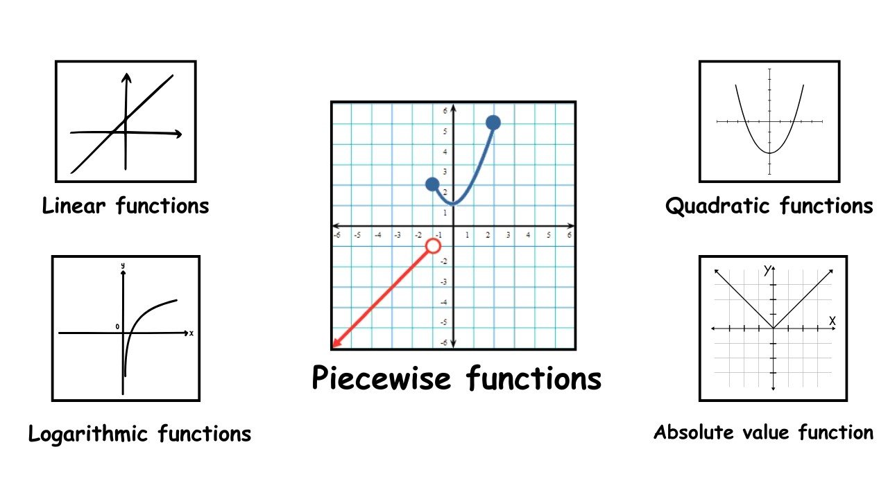
Piecewise functions are defined using different expressions depending on the interval of the domain in which x falls. This means the value of the function changes depending on the input range. For example, a piecewise function might equal −x + 2 if x ≤ −2, then x² − 1 if 0 ≤ x < 3, and −1 if x > 5.

These functions allow for modeling real-world phenomena that do not follow a single mathematical rule, such as electricity rates that change based on consumption, salaries with tiered bonuses, or physical systems that react differently depending on initial conditions. Analyzing this type of function requires examining each piece individually, evaluating continuity, differentiability, and break points. Although simple in definition, they can have very sophisticated applications in engineering, economics, and data science.

Further Reading

• Types of Functions on MathWorld
• Trigonometric Functions on MathWorld
• Hyperbolic Functions on MathWorld
• Floor and Ceiling Functions on MathWorld

---