
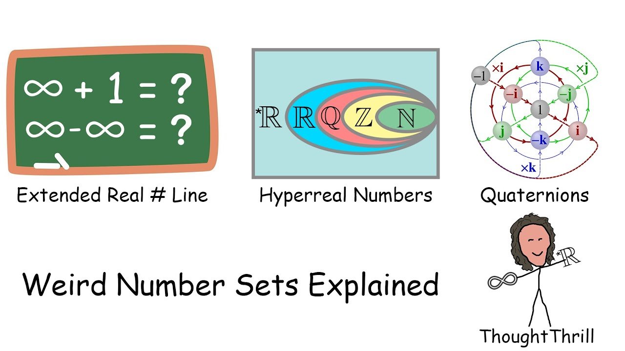
The Extended Real Number Line
We all know and love the real numbers. But infinity is not a real number, at least not in the mathematical sense of the term. Since this is math, though, we can make up new systems of rules if we want. In math, a rule that’s true because we say so is called an axiom. So let’s attach two endpoints to the real number line: positive and negative infinity. When we extend the real number line like this, what we get is the extended real number line.
Now, we aren’t quite done making up rules yet, because we need to decide what we can actually do with positive and negative infinity. Based on our current knowledge of numbers, let’s think about how we might want our new number system to work.
We know that a very big number plus a very big number is also a very big number. For example, 1 million plus 2 million equals 3 million. You can think about infinity as the biggest number there is. So if you add it to itself, that will also give you the biggest number there is, which is infinity again. So ∞ + ∞ = ∞. This may seem really silly and not very mathematical, but math and silliness are not mutually exclusive.
If you want to motivate this definition more rigorously, it’s certainly possible. For example, ∞ may be considered as the limit of a function whose value grows without bound. From there, the sum of two such functions can be shown to also grow without bound, yielding another infinite limit.
Now, a small number plus a big number is a big number. But every real number is small compared to ∞. So for every real number a, we can say that a + ∞ = ∞. But what if we add positive ∞ and negative ∞ together? If we add a very positive number and a very negative number, the result could be all sorts of things: a very positive number, a very negative number, zero, and so on. If you’ve taken calculus, you may recognize ∞ − ∞ as an indeterminate form of a limit, which similarly means that we can’t find a specific value without further information. Although it may seem reasonable to assume that positive ∞ and negative ∞ are both the same distance from zero and would therefore cancel out, we don’t do that here. So ∞ − ∞ is undefined.
Unfortunately, no, you still can’t divide by zero in this system. There is a system called the projectively extended real numbers that allows division by zero, but that’s a topic for another day.
You’ll recall that we were able to place number systems consisting of sets along with operations on them in categories like ring, semiring, and field. These are types of algebraic structures. So how can we categorize the extended real numbers together with addition and multiplication? It turns out that you can’t get very far. Addition and multiplication aren’t even binary operations in this system since they aren’t defined for all possible pairs of numbers. So our categorization system won’t work here.
Despite this, the extended real numbers can still prove to be useful. They can be used for limits, as doing arithmetic with ∞ can help simplify the process of figuring out what value a function is approaching. Limits are essential in calculus, and the extended real number system gives us a handy shortcut for calculating some of them.
The Hyperreal Numbers
Speaking of number systems involving some idea of infinity that can be useful in calculus, the hyperreal numbers are another example. In the case of the hyperreal numbers, in addition to ∞, we also have the inverse concept: infinitesimals, quantities considered to be infinitely small.
Before constructing the hyperreal number system, let’s figure out what we want to do with it. For the inventors of the system, the goal was to create a system that transferred the important rules of the real number system. Fittingly enough, this is called the transfer principle. In particular, we want this system with addition and multiplication to form a field, just like the real numbers.
With that in mind, let’s start by naming two of our new quantities. Omega (ω) is an infinite quantity, and epsilon (ε) is an infinitesimal quantity. Now we need some rules to distinguish these from ordinary numbers. The harmonic sequence, which is the sequence of reciprocals of positive integers (1/1, 1/2, 1/3, …), gets arbitrarily close to zero. So we can define an infinitesimal as a number whose distance from zero (or absolute value) is less than every element of the harmonic sequence. On the other hand, an infinite number is a number whose absolute value is greater than every positive integer.
Note that the reciprocal of a really big number is a really small number and vice versa. This behavior motivates us to state that ω and ε are reciprocals of each other: 1/ω = ε and 1/ε = ω. We can also use these two quantities in multiplication and addition. For example, you can have 7 + ε or 5ω. These are examples of hyperreal numbers. In this system, different sizes of infinities and infinitesimals can exist.
Finally, let’s introduce a special function: the standard part function, written as st. In simple terms, this function rounds a finite hyperreal number to the nearest real number. For example, consider the hyperreal number 12 + 5ε. Due to the 5ε term, this hyperreal number is an infinitesimal distance from the number 12. Applying the standard part function, we get st(12 + 5ε) = 12.
When applying this function to an infinite hyperreal number, we bring back the extended real numbers. An infinite hyperreal number has standard part positive or negative ∞ depending on its sign. For example, −3ω + 9 − 4ε is dominated by a negative infinite term, so the standard part is −∞.
The hyperreals can be used in calculus to obtain derivatives and integrals. This is called non-standard analysis, as opposed to the usual limit-based approach. In non-standard analysis, dx represents an infinitesimal difference in x, and the derivative can be defined directly in terms of infinitesimal ratios rather than limits. The hyperreals provide a useful alternative basis for calculus.
Increasing Dimensions: Why Not Three Components?
Let’s think about a different type of extension now. Not filling in the infinite endpoints on a number line, but rather increasing the dimension of our number system. We already know about the complex numbers, a system that extends the real numbers. Whereas the real numbers live on a one-dimensional line, the complex numbers live on a two-dimensional plane.
To be more precise about what we’re talking about, let’s think about how many real number components each type of number has. A real number obviously has one, and a complex number has two (the real and imaginary parts). Can we find a three-component number system? Say something like a + bi + cj for real a, b, and c.
It turns out that this ends up completely breaking things. In particular, just trying to find a value for ij can lead us to the conclusion that i = 1. So a + bi + cj reduces to (a + b) + cj, which is basically just a complex number with extra steps. This was the problem faced by Irish mathematician William Rowan Hamilton until he realized the solution in 1843 during a walk: use a fourth component. With that, he carved the equality i² = j² = k² = ijk = −1 into Broom Bridge, and the quaternions were born.
Quaternions
The most notable change when extending the complex number system to the quaternions is the loss of commutativity of multiplication. For example, ij = k, whereas ji = −k. Using our classification system, quaternions form a ring but not a field.
What can we do with quaternions? They turn out to be quite useful for several practical applications, like modeling rotations in three-dimensional space. We can summarize a treatment of quaternions using a geometric algebra perspective.
We have three perpendicular unit vectors e₁, e₂, and e₃. By the geometric product (which is associative but not commutative), eₘ² = 1 for all m, and eₘeₙ = −eₙeₘ for all m ≠ n. Multiplying two different unit vectors gives you a bivector, a plane segment oriented along the plane spanned by the two vectors you multiplied. Negating a bivector flips its orientation. Bivectors are considered rotation objects.
Let I = e₁e₂, J = e₂e₃, and K = e₁e₃. These, along with 1, are the basis elements of the quaternions. You can verify with the geometric product that this definition agrees with the defining equality from before.
Euler’s formula, e^(iθ) = cos θ + i sin θ, tells us how to rotate by angle θ, where eˣ is the exponential function. In 2D, for some vector v in the xy-plane, ve^(Iθ) rotates counterclockwise by θ, and e^(Iθ)v rotates clockwise. In 3D, rotation with either one alone distorts the e₃ coordinate. The solution is to rotate counterclockwise by θ/2 and also rotate clockwise by −θ/2, giving e^(Iθ/2) v e^(−Iθ/2). The bivector I can be replaced by an arbitrary unit bivector to rotate in any plane, working in any dimension. This gives the usual formula for quaternion rotation.
Further Reading
- Extended Real Number Line on MathWorld
- Hyperreal Numbers on MathWorld
- Quaternion on MathWorld
- Non-Standard Analysis at Stanford Encyclopedia of Philosophy
- Geometric Algebra on Wikipedia
Leave a Reply