
The Casas-Alvero Conjecture
If an integer k can be expressed as the product of two integers m and n, then m and n are called factors of k. A common factor of two integers is a factor shared by both. For instance, 4 and 6 have a common factor of 2.
Similarly, if a polynomial f can be expressed as the product of two polynomials g and h, then g and h are called factors of f. The polynomials x² + x and 2x + 2 have a common factor of x + 1, since they can respectively be expressed as x(x + 1) and 2(x + 1), where x, 2, and x + 1 are each polynomials of their own.
Now consider the single-variable polynomial function f(x) = x³ + 3x² + 3x + 1. This can actually be expressed as the third power of a polynomial of degree 1: f(x) = (x + 1)³. A polynomial of degree one is called a linear polynomial (some might call this “affine” instead, but this is just a difference in terminology).
Let’s take the derivative of our function. This can be factored into 3(x + 1)², showing that it shares a common factor of (x + 1) with f(x). Now take the second derivative of the original function. This factors into 6(x + 1), again sharing a common factor with f(x). Alternatively, you could have simply left the original function expressed as f(x) = (x + 1)³ and taken derivatives using the power and chain rules, which would have easily yielded the same result.
Now, the original function was of degree 3, and we’ve taken derivatives up to the second order, which is one less than 3. Therefore we can stop here. As we have seen, both of the derivatives share a common factor with the original function, and the original function can be expressed as a power of a linear polynomial.
The Casas-Alvero conjecture, proposed by Spanish mathematician Eduardo Casas-Alvero in 2001, is the hypothesis that whenever a polynomial f of degree d shares a common factor with all of its derivatives up to order d − 1, then f must be a power of a linear polynomial. The polynomials do not necessarily have to represent real numbers; they can represent the elements of any field of characteristic zero, of which the real numbers are an example.
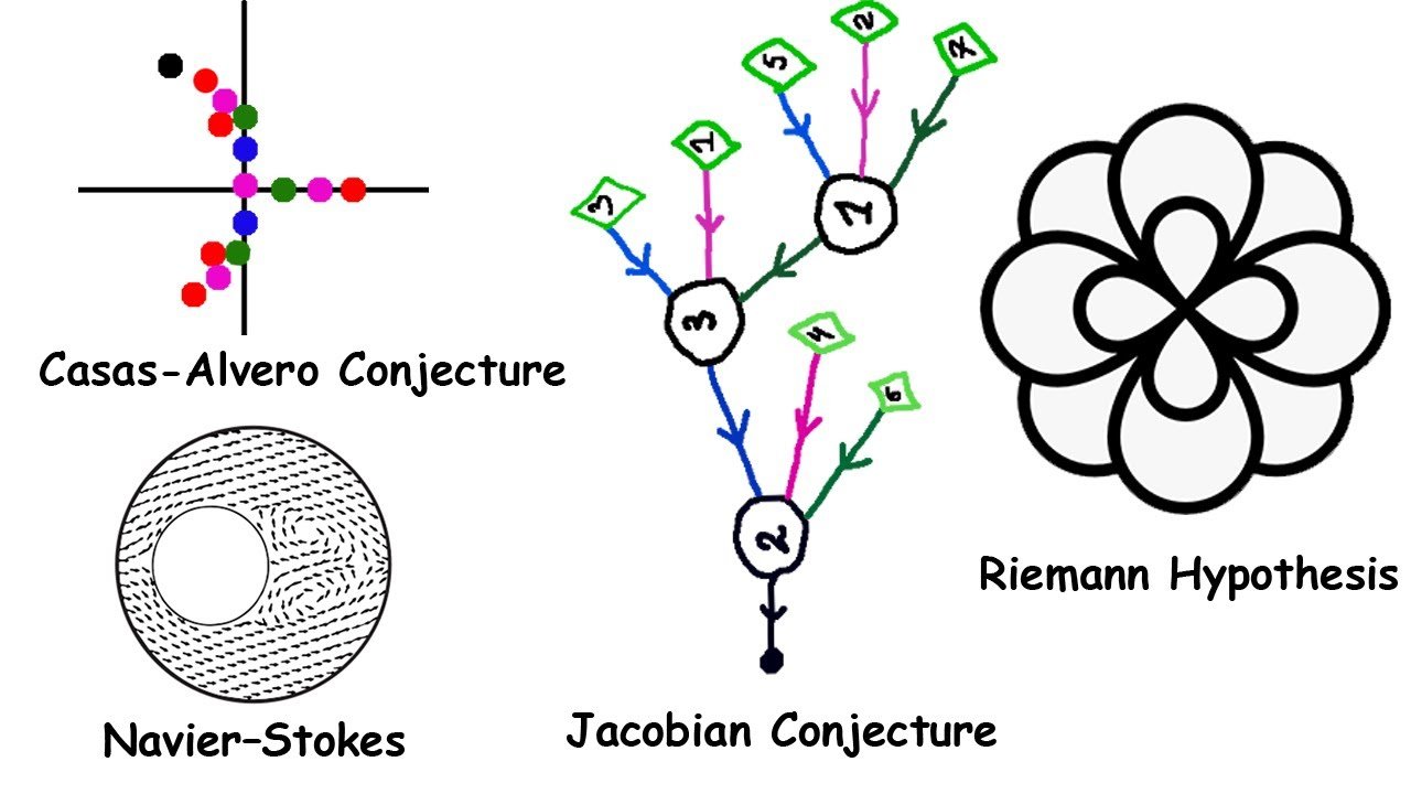
The Riemann Hypothesis
Take the sum 1/1ˢ + 1/2ˢ + 1/3ˢ + … toward infinity, where s is a complex number. An infinite sum like this is called a series. If the real part of s (the a in a + bi) is greater than 1, then this series converges, meaning that adding more and more terms makes it approach a specific finite value. We define the series to be equal to that value. This series is how the Riemann zeta function, named after German mathematician Bernhard Riemann, is defined for complex numbers with real part greater than 1.
On the rest of the complex plane, the Riemann zeta function is defined by filling in the gaps in a way where the function always has a derivative at every point where it’s defined. The complex derivative is defined similarly to the real derivative, just with everything being complex numbers. This method of extending a function is called analytic continuation. Using the portion we already have, there is exactly one way to do this, so we are locked into one specific definition for the function, even if the definition is very implicit. This defines the function for every complex number except s = 1.
Despite the relatively simple definition of this function, much remains unknown about it. In particular, one conjecture concerns the function’s zeros, the inputs where the function outputs a value of zero. Every negative even integer falls into this category, being called a trivial zero. Besides that, we know all other zeros have real parts between 0 and 1, occupying a region of the complex plane called the critical strip. The complex numbers with real part 1/2 compose a line called the critical line.
Riemann conjectured that all non-trivial zeros of the zeta function have real part 1/2, lying on the critical line. Indeed, this is true of every non-trivial zero found so far. This conjecture is known as the Riemann hypothesis, and proving or disproving it would have big implications in many areas of math. But no one has managed it. It is the sixth of the Millennium Prize problems, a set of problems with million-dollar prizes attached.
Navier-Stokes Existence and Smoothness
Consider the equation f′(x) = f(x). This states that the function f is its own derivative. An equation relating a function and its derivatives like this is called a differential equation. A differential equation can be solved, but instead of solving for a specific value, we are solving for the function f. Here the solution is f(x) = ceˣ for some constant c, as that captures every possible function, defined everywhere, which is its own derivative. Since the equation uses a single-variable function, it is called an ordinary differential equation, or ODE.
In contrast, multivariable calculus sees the use of multivariable functions like f(x, y) = x² + xy + y. You plug in two numbers x and y, and the expression on the right gives you a number in return. This concept gives rise to the partial derivative, a derivative with respect to one variable that treats the other variables as constants. An equation relating the partial derivatives of a multivariable function is called a partial differential equation, or PDE.
The Navier-Stokes equations are PDEs that characterize how viscous fluids move. They are named after Claude-Louis Navier and George Gabriel Stokes, the former a French engineer, the latter an Irish mathematician, both physicists.
The Navier-Stokes existence and smoothness problem, the fourth Millennium Prize problem, asks the following. Suppose you have an initial velocity field in 3D space, determining which way and how fast the particles in a fluid flow at the starting time. You need to prove that you can provide a vector velocity field and a scalar pressure field, both smooth and defined everywhere, that solve the Navier-Stokes equations. Or you need to provide an example of a case where this is impossible.
The Navier-Stokes equations are a promising lead when it comes to the concept of turbulence. Anyone who’s taken enough plane rides is probably familiar with turbulence. It’s when a fluid (as in a liquid or gas) rapidly undergoes chaotic changes, and it is one of physics’ biggest unsolved problems. Physicists believe that if we can understand the Navier-Stokes equations better, we will be able to understand turbulence better as a result.
The Jacobian Conjecture
In multivariable calculus, a function can take in a vector and give you a vector in response. For instance, you can have the function f(x, y) = (2y, 3x). Evaluating this function on the vector (1, 2), you get f(1, 2) = (2 × 2, 3 × 1) = (4, 3). So the vector (1, 2) gets mapped to (4, 3). Here the first part of the output, f₁ = 2y, is called the function’s first component, and the second part, f₂ = 3x, is called the second component.
When you have a function like this, you can construct its Jacobian matrix. This is a matrix filled with each of the partial derivatives of each of the components of f. In our case, with two input variables and two output components, we can evaluate it as a 2 × 2 matrix. Since our input and output have the same number of dimensions, the matrix we get is a square matrix. This means that we can take its determinant, called the Jacobian determinant, denoted Jf.
The formula for the determinant of a 2 × 2 matrix is ad − bc, which we can apply to our matrix. For our example, the Jacobian determinant turns out to be −6.
The Jacobian matrix and determinant are named after German mathematician Carl Gustav Jacob Jacobi. They allow us to apply linear algebra concepts to transformations of space that look locally linear in a small neighborhood of each point.
The other concept needed is that of a field, which is a set equipped with the normal arithmetic operations with similar behavior as in the real numbers. A field has an additive identity and a multiplicative identity. Adding the additive identity doesn’t change an element, nor does multiplying by the multiplicative identity. These are 0 and 1 in the real numbers, respectively. If the additive identity can’t be obtained by adding together a positive number of copies of the multiplicative identity, the field is said to have characteristic zero. You can’t add a positive number of ones to get zero, so the real numbers have characteristic zero.
Now let K be a field of characteristic zero, and let f be a function from Kⁿ to itself, for fixed integer n greater than 1. For example, K could be the real numbers and n could be 2. Then f would map from ℝ² to itself, where ℝ² is the usual 2D vector space.
The Jacobian conjecture states: if Jf is some constant nonzero value, then f has an inverse function g with polynomial components.
To use our earlier example, we found that the Jacobian determinant of our function was −6, which is indeed a constant and also not zero. Can we find an inverse g that maps the output back to the input? That involves solving the equation (2y, 3x) = (a, b) for x and y, yielding g(a, b) = (b/3, a/2). Both b/3 and a/2 are indeed polynomials, so g does have polynomial components.
If you can either prove or disprove that this will always happen, you will have solved the Jacobian conjecture.
Further Reading
- Riemann Hypothesis on MathWorld
- Navier-Stokes Equations at the Clay Mathematics Institute
- Jacobian Conjecture on MathWorld
- Casas-Alvero Conjecture on Wikipedia
- Analytic Continuation on MathWorld
Leave a Reply