Every Important Graph in Math Explained

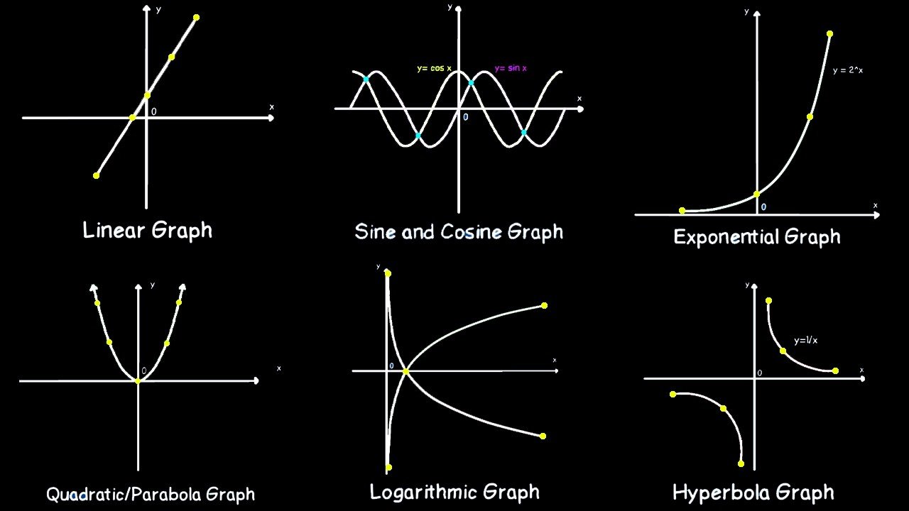
Linear Graphs

A linear graph is a line-shaped graph that can be written as y = mx + b. Here, m is the slope: for every one unit you go to the right, you rise by m units. And b represents the y-coordinate of the y-intercept, which is the point where the graph crosses the y-axis. This can be found by setting x equal to 0 in the equation y = mx + b, which gives y = m × 0 + b, or y = b. Because the form y = mx + b directly gives the slope and the y-intercept of the graph, it is called slope-intercept form. A linear function is a special case of a polynomial function: it is a first-degree polynomial.

It is also possible to write an equation for a linear graph given its slope m and a point that it passes through, (x₁, y₁). We begin with the equation y = mx, which gives us a line of slope m passing through the origin. We can shift it vertically by y₁ by replacing y with y − y₁, giving y − y₁ = mx. Then we can shift it horizontally by x₁ by replacing x with x − x₁, giving y − y₁ = m(x − x₁). Overall, shifting the line has the effect of moving it to intersect the point (x₁, y₁), where that point basically acts like the origin did. This form of the equation is known as point-slope form.

The final common form is called standard form, which is ax + by = c, where a, b, and c are integers. This form separates the variable terms from the constant term. However, note that some linear equations can’t be rewritten in standard form with integer coefficients, like y = √2 · x.

Linear equations are used to model variables with a constant rate of change. For example, the velocity of a falling object (under constant acceleration) is proportional to the time it has fallen, so the graph of a falling object’s velocity over time is a straight line.

Quadratic Graphs

A quadratic graph comes from a second-degree polynomial function y = ax² + bx + c. Every quadratic graph is a parabola, which is a roughly U-shaped curve. If a is positive, then the parabola opens upward. If a is negative, then the parabola opens downward. The greater the magnitude of a, the more sharply the parabola bends.

The graph of a quadratic function can help you find the points where the function attains a value of zero, often simply called the zeros or roots of the function. Equivalently, these are the points where the graph intersects the x-axis. In general, for a quadratic function there are three cases to consider. First, two x-axis intersections: the function has two real-valued zeros, each with multiplicity one, and the discriminant b² − 4ac is positive. The discriminant is the value inside the square root in the quadratic formula, x = (−b ± √(b² − 4ac)) / 2a. Second, one x-axis intersection: the function has one real-valued zero with a multiplicity of two, meaning the discriminant equals zero. Third, no x-axis intersections: the function has no real-valued zeros (its zeros exist only in the complex numbers), and the discriminant is negative.

Quadratics have many uses in modeling real-world phenomena. One of the simplest examples is parabolic motion: a projectile, an airborne object with no forces acting upon it except gravity, traces out the shape of a parabola as it flies through the air. A parabola is an example of a conic section, which is, roughly speaking, the intersection between an infinitely large cone and a plane slicing through it.

Circles

The equation for the graph of a circle is (x − h)² + (y − k)² = r², where r is the radius and (h, k) is the center of the circle. This equation can be derived from the definition of a circle and the Pythagorean theorem.

A circle is defined as the set of all points in a plane that are at an equal distance (the radius) from a given point (the center). For the simplest case, imagine a circle centered at the origin. Draw a radius line segment from the center of the circle to some point on the circle. This line segment’s length is r. Now say that the point on the circle has coordinates (x, y). Draw a vertical line segment from that point to the x-axis, then draw a line segment from the point you reached back to the origin. The three line segments form a right triangle. The lengths of its legs are x and y, and the length of its hypotenuse is r. Now we can just apply the Pythagorean theorem: x² + y² = r².

So we know that this equation captures that particular point on the circle. But there’s nothing special about the point we chose. We can do the exact same thing for all of the infinitely many points of the circle. Thus x² + y² = r² defines a circle of radius r centered at the origin.

To generalize this so the circle can be anywhere in the plane, we must think about graph transformations. Replacing x with x − h shifts the graph h units to the right. Similarly, replacing y with y − k shifts the graph k units upward. So to center the circle at the point (h, k), we use (x − h)² + (y − k)² = r².

One important case is the circle of radius 1 centered at the origin, given by x² + y² = 1. This circle is the basis of the trigonometric functions sine and cosine. If you start at the right of the circle and travel some distance θ counterclockwise around the unit circle, then sin θ gives you your y-coordinate and cos θ gives you your x-coordinate.

Ellipses

Similarly to a circle, an ellipse is defined using distances from points. In the ellipse’s case, it uses two points, each of which is called a focal point or focus (plural: foci). An ellipse is defined as follows: if you choose any point on the ellipse, take the distances from that point to each of the focal points, then add those distances up, you will always get the same number, no matter which point you choose. Thus the ellipse is a generalization of the circle, which is simply the special case where the two focal points are the same point. An ellipse can also be thought of as a stretched-out circle.

The equation for an ellipse centered at the origin with a width of 2a and a height of 2b is x²/a² + y²/b² = 1. The farthest points on the ellipse from the center are called the vertices, and the closest points are called the co-vertices. A line segment from the center to a vertex is called a semi-major axis, and one from the center to a co-vertex is called a semi-minor axis. The distance c from the center to a focus is called the ellipse’s linear eccentricity, and the value e = c/a is its eccentricity. Like a parabola, an ellipse is also a conic section.

Hyperbolas

A hyperbola is a curve consisting of two roughly U-shaped pieces, or branches, bending away from each other. It can be defined in various ways, including as a conic section like the parabola and the ellipse. It can also be defined using two focal points, just like the ellipse, only using the absolute difference of the distances rather than the sum.

A hyperbola centered at the origin can be given the following equations: x²/a² − y²/b² = 1 or y²/a² − x²/b² = 1. This is similar to the equation for the ellipse but with subtraction instead of addition. If x is in the first term, the hyperbola opens sideways. If y is in the first term, the hyperbola opens up and down. The two points of the hyperbola closest to its center are called its vertices. The line segment between these vertices is called the transverse axis.

The hyperbola has two asymptotes, where an asymptote is a line that you get closer and closer to as you approach infinity. The unit hyperbola is given by x² − y² = 1. It is the basis of the hyperbolic functions sinh (hyperbolic sine) and cosh (hyperbolic cosine), which are analogous to the ordinary trigonometric functions. If you draw a line segment from the center to a point on the right half of the unit hyperbola, then the signed area bounded by the line segment, the hyperbola, and the x-axis is denoted by a/2. Signed area means that if the area is below the x-axis, it’s counted as negative. The point where your line segment hits the unit hyperbola has coordinates (cosh(a), sinh(a)).

Sine and Cosine

Sine and cosine are two of the basic trigonometric functions. They give the coordinates of a point on the unit circle given a distance θ that it has traveled around the circle. The graphs of sine and cosine look like waves, swinging up and down between −1 and 1 forever, which reflects the functions’ cyclical nature. Waves of this form are known as sinusoidal waves. Due to this swinging behavior, they do not have a limit as their input reaches infinity.

The period of the sine function, or the amount of time it takes to complete one cycle, is 2π (also known as τ, the ratio of a circle’s circumference to its radius, about 6.28). At θ = 0, sin θ = 0. Then at θ = π/2 (one quarter of the way around the unit circle), sin θ reaches a maximum value of 1. At θ = π (halfway around), sin θ returns to zero. At θ = 3π/2, sin θ reaches a minimum of −1. And at θ = 2π (all the way around), sin θ is back to zero again, and the sine function has completed a full cycle.

Similarly, the cosine function also has a period of 2π. At θ = 0, cos θ = 1. At θ = π/2, cos θ = 0. At θ = π, cos θ = −1. At θ = 3π/2, cos θ = 0. And at θ = 2π, cos θ = 1.

Exponential Functions

An exponential function is a function of the form y = aˣ. This can be used to model either exponential growth or exponential decay, depending on whether a is greater than or less than 1.

For a > 1, the function grows as its input increases. It approaches zero on the left and rises toward infinity on the right. Meanwhile, for 0 < a < 1, the function does the reverse, trending downward from positive infinity on the left and decaying asymptotically toward zero on the right. This corresponds to the fact that repeatedly multiplying a number bigger than 1 by itself will give you a bigger number, but for a number less than 1, you’ll get a smaller number.

If you plug in a = 1, you get y = 1ˣ, which just reduces to y = 1, so it doesn’t grow or decay in either direction. You can also plug in a = 0 to get y = 0ˣ. This breaks into three parts: for x > 0, the value is 0; for x < 0, the expression is undefined (you can’t raise 0 to a negative power); and for x = 0, that would require evaluating 0⁰, the value of which is not universally agreed upon. It is conventionally either given the value of 1 or left undefined.

In calculus, the most important exponential function is y = eˣ, where e is Euler’s number. The function eˣ is its own derivative: the rate of change at each point is the same as the value of the function at that point, so d/dx of eˣ = eˣ. Due to this, it is also its own antiderivative, so it can be obtained by integrating itself. In terms of the graph, this means that at any given point, the height above the x-axis, the slope of the tangent line, and the area under the curve from −∞ to that point are the exact same value.

Logarithmic Functions

A logarithm, denoted by log, is an inverse function to an exponential function. Essentially, for any appropriate a and x, log_a(aˣ) = x, where a is called the base of the logarithm. In calculus, similarly to how eˣ is the most important exponential function, the logarithm with base e is the most important logarithmic function. This logarithm has a special name: the natural logarithm, usually denoted by ln. Other frequently used logarithms are the common logarithm (base 10) and the binary logarithm (base 2), with the latter being common in computer science.

The graph of any inverse function can be created by taking the graph of the original function and reflecting it across the line y = x. For the natural logarithm, what we get is a curve that shoots up from negative infinity just to the right of x = 0, crosses the x-axis at x = 1, and then grows more and more slowly as it goes to the right. However, its growth is unbounded, so it will reach arbitrarily high values if you go far enough. We can also graph the common logarithm, which has a bigger base so it grows more slowly, and the binary logarithm, which has a smaller base so it grows faster.

You can also use a base between 0 and 1 for the logarithm. This results in a graph that plummets from positive infinity, crosses through the x-axis at x = 1, and decreases more and more slowly forever. If you replace the base of a logarithm with its reciprocal, this has the effect of flipping the graph across the x-axis. For example, the graph of log₁/₂(x) is just a flipped version of log₂(x).

The natural logarithm is important in calculus because its derivative is y = 1/x. Correspondingly, by integrating this function, you can get the natural log: ln(x) = ∫₁ˣ (1/t) dt. This is one possible definition of the natural logarithm.

This article was generated from the video transcript of “Every Important Graph in Math Explained”.
Watch the full video above for visual explanations and diagrams.