
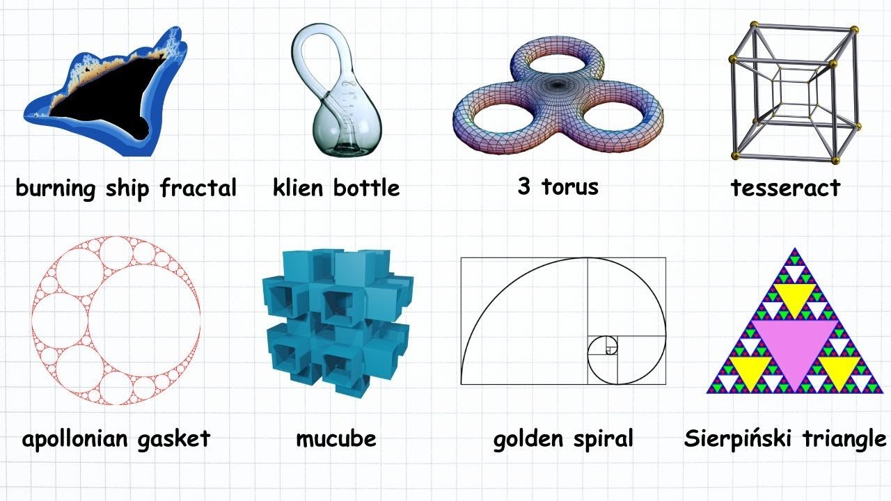
The Apollonian Gasket
Let’s start by drawing a circle named C₁. Note that we’re not including the inside region as part of the circle. That region is called a disc in math terms. Now draw a second circle C₂ that touches C₁ at just one point. These circles are tangent to each other. You can even draw it so that either circle is inside the other if you want. Now draw a third circle C₃ tangent to both of the first two. Just make sure that it’s not tangent at the same point where C₁ and C₂ are tangent to each other.
Now that we have these three circles, we can always draw exactly two more circles that are tangent to all of the first three. This was discovered by the ancient Greek mathematician Apollonius of Perga, who lived from roughly 240 BC to 190 BC. Because of this, when five circles are arranged in this way, they are called Apollonian circles in his honor.
Now that we have these five circles, let’s keep drawing even more. Inside the largest circle, but outside all the circles contained within, there are six gaps that look like curved triangles. We can draw another circle inside each of these gaps, making the new circle tangent to each of the neighboring circles. Once we are done, we have created 18 new triangular gaps, which we can fill with tangent circles as well. We can just keep repeating this process on and on forever. In the limit, we get an infinitely detailed shape, a fractal. This particular fractal is called the Apollonian gasket.
The Golden Spiral
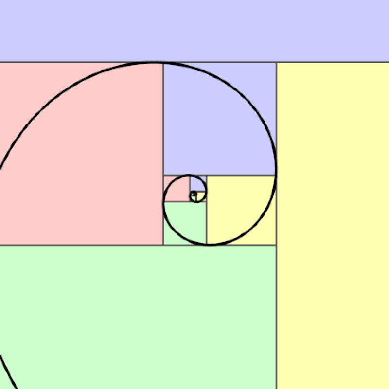
Suppose you have two amounts, and the ratio of the larger amount to the smaller amount equals the ratio of the sum of the amounts to the larger amount. In that case, this ratio will always be the same special number: the golden ratio, denoted by the Greek letter φ (phi). If we call the larger amount a and the smaller amount b, the golden ratio can be expressed by the equality a/b = (a + b)/a. It equals (1 + √5)/2, about 1.618.
You may know about Cartesian coordinates, x and y, where x tells you how far horizontally to go and y tells you how far vertically. Another way to label points in 2D space is polar coordinates. Starting from the origin, which is now called the pole, draw an infinite ray toward the right called the polar axis. This system has two coordinates, r and θ. To reach a point, stand at the pole and face along the polar axis, rotate an angle of θ counterclockwise, then walk a distance of r forward. For instance, if the coordinates are (r, θ) = (3, 90°), then rotate 90° counterclockwise and walk 3 units forward.
Mathematicians prefer using radians rather than degrees. The number of radians in a full turn is 2π (also known as τ, tau), which is about 6.28. Since 90° is a quarter turn, that’s τ/4 radians, so the coordinates (3, 90°) can be rewritten as (3, τ/4).
In Cartesian coordinates, an equation can describe a set of points, like y = 1 or y = x. Similar equations are possible in polar coordinates, like r = 1 or r = θ. Let’s examine r = 2^θ, which generates a spiral shape. By definition, this can be rewritten as θ = log₂(r). This is an example of a logarithmic spiral. The logarithm can be any base, and you can multiply r by a constant. One example is θ = ln(3r), also written r = (1/3)e^θ, where e is Euler’s number, about 2.718.
Now imagine a logarithmic spiral that grows by a factor of φ each quarter turn. We want φ as the base of exponentiation, and each quarter turn should increase the exponent by 1. That gives us r = φ^(θ/(τ/4)). And with that, we have the golden spiral.
The Torus
A torus is simple. It’s just a donut shape. Note that the torus is hollow. If the inside is included, it’s called a solid torus instead.
Now let’s imagine the torus is actually a space. Consider a creature living on the torus. Just as we can never leave our own space, this creature cannot ever leave the torus. However, it is free to move along the torus, and it has two degrees of freedom to do so. This is similar to a plane, which also allows two degrees of freedom. Therefore, the torus is topologically two-dimensional.
One way to construct a torus is to start with a rectangle. Glue one pair of opposite edges together to form a tube, and then glue the ends of the tube together. Of course, the rectangle should be made of an elastic material for this to work properly. You could simply imagine the creature moving around on this rectangle, looping around when it reaches an edge. If it keeps traveling upward, it’ll just loop back to where it began. The same for traveling rightward. The creature’s universe is finite but has no boundary.
We can do a similar thing for a 3D object, a solid cube. However, this requires stretching and folding the cube up into a higher dimension, so it’s harder to visualize. Nevertheless, we can glue each pair of opposite faces of the cube together, similarly to what we did for the rectangle. The shape we get is called a 3-torus. Since you are a 3D creature, you can imagine yourself living in this space. Similarly to how the 2D creature could not see the seams while living in the 2-torus, you cannot see the walls of the cube while living in the 3-torus. In fact, they do not really exist to you. Within the 3-torus, you can simply travel forward in a straight line and loop back on yourself.
In terms of our own universe, much remains unknown about its shape. Multiple different hypotheses have been proposed. One possibility is that it simply loops back on itself forever, just like the 3-torus.
The Mucube
Think of the usual polygons: triangles, quadrilaterals, pentagons, and so on. Using these polygons in 3D space, you can join their edges to form a 3D shape known as a polyhedron. Each polygon is called a face of the polyhedron. If all of the polyhedron’s vertices, edges, and faces are the same (more precisely, if you can move each vertex, edge, or face to any other of the same type while keeping the polyhedron identical), it is called a regular polyhedron.
Imagine cutting off a corner of a polyhedron and looking at the cross-section. The shape you see is known as a vertex figure. For instance, if you cut off the corner of a cube, the shape you get is a triangle. The number of angles of the vertex figure is always equal to the number of edges of the polyhedron that join at the vertex.
Now, the vertices of a polygon usually lie in the same flat space, or plane. In other words, they are coplanar. However, it is possible to have a polygon with non-planar vertices, known as a skew polygon. A polyhedron may be made out of skew polygons, or it may have a skew polygon as a vertex figure. In that case, it is called a skew polyhedron. In particular, it is called a regular skew polyhedron if the skew polygons in question are regular. An infinite regular skew polyhedron is called a regular skew apeirohedron.
Now imagine an infinite grid of cubes, known as a cubic honeycomb. If you remove two opposite faces from each cube in a certain way, you will get a special shape called a mucube (short for “multiple cube”). Any vertex, edge, or face of the mucube can be moved to any other while keeping it the same, so it is a regular polyhedron, specifically a regular skew apeirohedron.
The Burning Ship Fractal
You may recall the definition of the Mandelbrot set from earlier. Just to quickly recap: we choose a complex number c and define a complex function f_c with the equation f_c(z) = z² + c. Starting with z = 0, we apply this function over and over again. If we get a sequence that doesn’t diverge to infinity, then we include the number c as a member of the Mandelbrot set.
The burning ship fractal is defined in a very similar way. The function is almost the same, but before we take the square, we first set the real and imaginary parts to their absolute values. That results in a modified function.
Let’s go through an example. Suppose we have the complex number z = −3 − 2i. The real part is −3 and the imaginary part is −2. Replacing each of these with their absolute value, we get 3 + 2i. This can be represented graphically in the complex plane: we flip −3 − 2i across the vertical axis and then across the horizontal axis so that it ends up in the upper right quadrant. Meanwhile, if we had started with a number like 4 + 5i, that would remain the same because taking the absolute values of each part doesn’t change their value.
The rest of the process is just like the Mandelbrot set. We start by selecting a value of c. Then we apply the function over and over, starting with z = 0. If the value stays bounded, then c is in the burning ship. Drawing all such values and coloring other values based on their speed of divergence (and vertically flipping the image because it looks nicer), we get the burning ship fractal.
The Sierpiński Triangle
Take three identical equilateral triangles and join them at the vertices so that they form another equilateral triangle in the middle. Then shrink this shape down by a factor of 1/2. Take three identical copies of it and join them in a similar way. If you do this process over and over again, the shape you approach is called the Sierpiński triangle, named after Polish mathematician Wacław Sierpiński.
The Sierpiński triangle is an example of a fractal, a shape that has infinite detail. No matter how far you zoom in, it never smooths out. In particular, the Sierpiński triangle is a self-similar fractal. It is composed of three smaller copies of itself.
The study of fractals also gives rise to the idea of fractal dimension. A line segment is considered one-dimensional, a square is two-dimensional, and a cube is three-dimensional. If you scale up the dimensions of each of these by a factor of 2, then the line segment’s length is scaled by 2¹ = 2, the square’s area is scaled by 2² = 4, and the cube’s volume is scaled by 2³ = 8. In each case, the exponent is equal to the dimensionality of the object.
If you scale up the dimensions of the Sierpiński triangle by a factor of 2, it becomes 3 times as large. As a result, its dimensionality d can be found by solving 2^d = 3. Taking the logarithm base 2 of both sides, we see that d = log₂(3), which is about 1.585. In this sense, the Sierpiński triangle is approximately 1.585-dimensional. This is called its Hausdorff dimension, named after German mathematician Felix Hausdorff.
The Tesseract
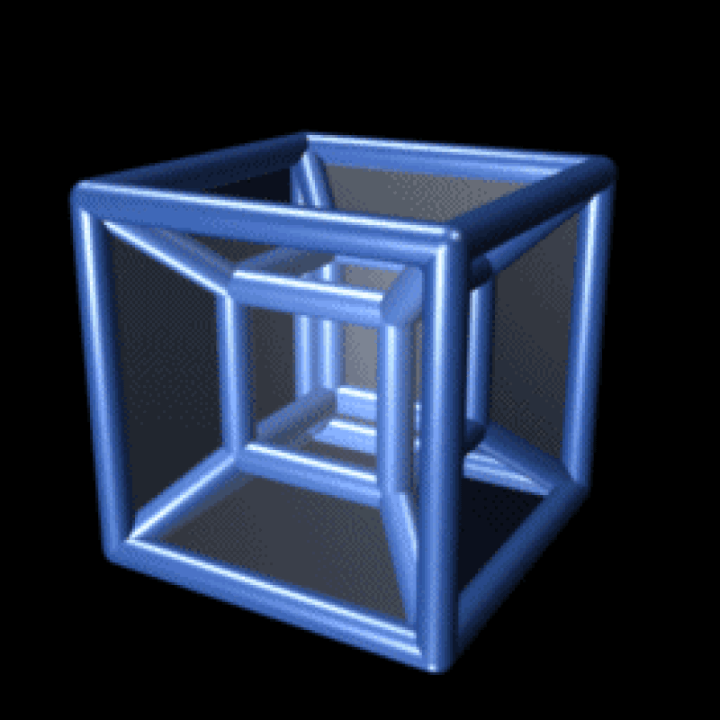
The tesseract is the four-dimensional analog of the cube. Just as a line segment is formed by connecting two points, a square by connecting four line segments, and a cube by connecting six squares, a tesseract is formed by connecting eight cubes. These eight cubes are called the facets of the tesseract. For each dimension n, the analog of the cube is known as the n-dimensional hypercube.
Four-dimensional shapes are difficult to visualize in a world with only three dimensions of space. However, one option is to look at a 3D projection. Just as the 2D projection of a 3D object can be thought of as its 2D shadow, the 3D projection of a 4D object can be thought of as its 3D shadow.
Just like the cube has a volume and a surface area, the tesseract has a 4D hypervolume. For a side length s, the length of a line segment is s, the area of a square is s², and the volume of a cube is s³. Accordingly, the hypervolume of a tesseract is s⁴. The surface area of a cube is obtained by adding together the areas of its six square facets, yielding 6s². Likewise, the surface volume of a tesseract is obtained by adding together the volumes of its 8 cubic facets, yielding 8s³.
The Klein Bottle
Let’s start with a Möbius strip, named after German mathematician August Ferdinand Möbius. This is a standard object that you could make at home. Just take a paper strip, give one end a half twist, and attach the ends together. This results in a piece of paper with just one side.
The Möbius strip is a nonorientable surface, meaning that clockwise and counterclockwise rotation cannot be distinguished within it. If you imagined yourself traveling along the length of the Möbius strip, upon returning to your starting point you would find yourself upside down from your starting orientation. Of course, this supposes that you’re a 3D object traveling on top of the Möbius strip. But if you’re actually a 2D object living within it, then traveling along it back to your starting position would cause you to become your mirror image. Accordingly, rotations that once looked clockwise would now look counterclockwise. So an orientation cannot be consistently defined for this surface.
The Klein bottle, named after German mathematician Felix Christian Klein, is another example of a nonorientable surface. However, it has no boundary, meaning there are no points where the surface abruptly stops. It does not intersect itself, though it often seems to in visualizations due to the limitations of 3D space. In 4D space it is easily constructed from the Möbius strip. Just take two copies of the Möbius strip and glue their edges together.
Or, in the words of Austrian-Canadian mathematician Leo Moser: “A mathematician named Klein / Thought the Möbius band was divine. / Said he, ‘If you glue / The edges of two, / You’ll get a weird bottle like mine.’”
The Mandelbrot Set
The Mandelbrot set, named after French-American mathematician Benoît B. Mandelbrot, arises in the study of complex numbers. We begin by picking some number c in the complex plane. Using c, we define a complex function f_c(z) = z² + c. Basically, this function takes in a number, multiplies it by itself, adds c, and spits out the result.
Start by evaluating this function at z = 0. For instance, if you chose c = 1, then f₁(0) = 0² + 1 = 1. Then take the result and plug it back into the same function: f₁(1) = 1² + 1 = 2. Keep doing this over and over again.
Depending on the value you chose for c, the resulting sequence of numbers may stay bounded in absolute value or it may diverge toward infinity. In our c = 1 case, it diverges since the sequence goes 0, 1, 2, 5, 26, and so on. The Mandelbrot set is the set of all possible values of c you could choose that result in a bounded sequence. As we saw, the number 1 is therefore not an element of the Mandelbrot set, but the number −1 is, since that produces the bounded sequence 0, −1, 0, −1, 0, and so on.
The Mandelbrot set is contained entirely within the disc of radius 2 centered at the origin, and its boundary has Hausdorff dimension 2. If you draw the Mandelbrot set in the complex plane, you get a very intricate shape, infinitely intricate in fact, making it a fractal. Zooming in, we see that it is a self-similar fractal at certain points, and a variety of other patterns can be found. Due to its intricacy, the Mandelbrot set has been cited as an example of mathematical beauty, particularly how complex patterns can arise from simple definitions.
The Weierstrass Function
In calculus, you may know about the concept of a differentiable function. If you take the graph of a function and zoom in at a certain point, it may straighten out, looking more and more like a line. If it does, then the line being approximated is called the tangent line. If this line is not vertical, then the function is differentiable at that point, and the derivative is the slope of the tangent line.
In order for a function to be differentiable at a point, it must be continuous there, meaning you can draw its graph without picking up your pencil. Also, it cannot bend sharply there. For example, the absolute value function is not differentiable at zero. No matter how far you zoom in on its graph at x = 0, it never straightens out.
It is easy to imagine a continuous function that is non-differentiable at a finite, or even countably infinite, number of points, since that just means the graph has a sharp bend there. However, it is much harder to imagine a continuous function that’s infinitely jagged and doesn’t smooth out anywhere. Thus, for a long time, mathematicians assumed that there was no function that is continuous everywhere and differentiable nowhere.
The Weierstrass function is a function that is continuous everywhere and differentiable nowhere. It was discovered by German mathematician Karl Weierstrass and first published in 1872. Weierstrass defined it using an infinite sum called a Fourier series. Here, a must be strictly between 0 and 1, b must be a positive odd integer, and ab must be greater than 1 + 3π/2. Whatever values you pick for a and b that follow these rules, you will get the same qualitative behavior.
The graph of the Weierstrass function is a self-similar fractal curve. However, such curves were hard to visualize back then. The existence of the Weierstrass function destroyed several proofs that relied on continuous functions being differentiable almost everywhere. So it was denounced by mathematicians at the time. Later, the mathematical community came to the realization that counterintuitive facts can be true, and the Weierstrass function is widely accepted today.
Seifert Surfaces
Take a long piece of rope and arrange it into whatever form you like. Then glue together the two dangling ends. Mathematically, the resulting object is known as a knot. If you can stretch and squish one knot into another without using self-intersections, then the two knots are the same. If you take a combination of one or more knots, where these knots may or may not be separable, you get an object called a link. Knots and links are important objects of study in the mathematical field of knot theory.
The simplest knot is the unknot, which is basically just a loop of rope without anything being tied. The next simplest knot is the trefoil knot, which can be created by connecting the ends of an overhand knot. As for links, an unlink is any finite collection of circles that aren’t connected together at all. The Hopf link, named after German mathematician Heinz Hopf, consists of two circles linked together. And the Borromean rings, named after the aristocratic Borromeo family, are three linked circles that fall apart if any one is destroyed.
A Seifert surface, named after German mathematician Herbert Seifert, is an orientable surface with a boundary that is a knot or link. The simplest example is a disc, which is a surface whose boundary is a circle (which is just an unknot). Noting the requirement of orientability in the definition, the Möbius strip is not a Seifert surface even though its boundary is an unknot. A Seifert surface formed by a Hopf link may resemble a Möbius strip, but it is actually topologically equivalent to an annulus (the planar region bounded by two concentric circles) and is thus orientable. A Seifert surface formed by the Borromean rings has its own beautiful and intricate shape.
Further Reading
- Apollonian Gasket on MathWorld
- Golden Ratio on MathWorld
- Mandelbrot Set on MathWorld
- Sierpiński Triangle on MathWorld
- Weierstrass Function on MathWorld
- Klein Bottle on MathWorld
- Seifert Surface on MathWorld
Leave a Reply