
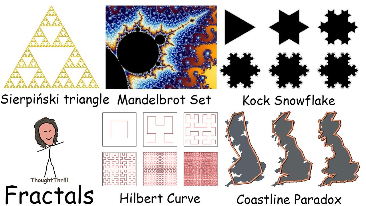
Fractals are geometric objects that have a fascinating property: they are self-similar. This means that their structure repeats itself at different scales, no matter how close or far away you are looking. Imagine an object whose shape repeats itself over and over again, just at different sizes. These structures are not just abstract objects but are found in nature, science, and art. Some examples are tree branches, lightning, octopus tentacles, leaves, ferns, peacock feathers, snail shells, snowflakes, Romanesco broccoli, The Great Wave of Kanagawa, lungs, neural networks, river networks, and coasts.
Characteristics of Fractals
Fractals have several characteristics that distinguish them from traditional geometric figures:
Self-similarity: A structure that is repeated at different scales.
Fractal dimension: The dimension of a fractal is not an integer, as in conventional geometric figures, but a fractional number that describes the complexity of the fractal.
Infinite complexity: Although fractals are generated by simple rules, their complexity is infinite. That is, they can continue to develop in smaller details without ever reaching a completely detailed resolution.
Infinite perimeter and finite area: Fractals can have an infinite perimeter while maintaining a finite area.
Fractal dimension does not refer to the number of dimensions in the traditional sense, but to how the object behaves as we scale it. The more the pattern repeats at different scales, the larger the fractal dimension. Traditional geometric figures such as a square and a line have integer dimensions of two and one respectively. Fractals have fractional dimensions.
Hausdorff Dimension
Hausdorff dimension is a metric generalization of the concept of dimension of a topological space. Let’s consider the following line (red), which can be formed by three segments (orange, blue, green). This means that to form the original line (red), it is necessary to fill the space with three segments. This, according to Hausdorff’s definition, translates to n = L^D, where D equals Euclidean dimension, n equals self-similar objects needed to cover the original object, and L equals reduction factor.
Using properties of logarithms, we have log(n) = log(L^D). Clearly, n has to be based on L, so D = log(n)/log(L).
In the case of the straight line, it is D = log(3)/log(3) = 1.
Now let’s consider the square. It takes nine segments to fill the space of the original square (red). That is, D = log(9)/log(3) = 2.
The Mandelbrot Set
Now let’s talk about the most famous fractal: the Mandelbrot set. The mathematical definition of the Mandelbrot set consists of iterating a mathematical function over each point in the complex plane and seeing if the resulting sequence stays within a limit or moves away towards ∞. Points that stay within the limits form the famous head of the Mandelbrot set, while points that move away towards ∞ create the infinite details as we zoom in.
The most impressive thing about the Mandelbrot set is its self-similarity. As we get closer to the edges of the set, we discover that the same patterns are repeated over and over again, but with infinitely small details. It is a fractal in all its glory.
Koch Snowflake
Another well-known fractal is the Koch snowflake. This fractal is built iteratively, starting with an equilateral triangle. At each step of the iteration, each side of the triangle is cut away and replaced by a new set of three line segments that form a peak. This process is repeated infinitely, creating an increasingly complex figure.
By applying a reduction factor of three, it is possible to identify four segments of equal length. This is known as the first iteration, and it is possible to identify the fractal dimension: D = log(4)/log(3) = 1.2618. The following iterations of the Koch snowflake continue this pattern through iteration 2, iteration 3, iteration 4, iteration 5, and iteration 6.
Sierpiński Triangle
The Sierpiński triangle is a fractal created from an initial equilateral triangle. At each iteration, a central triangle is removed, leaving three smaller triangles in its place. This process is repeated infinitely, creating a figure that is completely self-similar.
Let’s consider the original triangle. For this, a reduction factor of two is applied. That is, each side of the triangle intersects in the middle of each segment by creating three new triangles. The center triangle is eliminated. We have reduced a quarter of the original area of the triangle, which implies that for a reduction factor of two, three new elements have been created. Therefore, the fractal dimension of the Sierpiński triangle is D = log(3)/log(2) = 1.5849.
Like every fractal, the Sierpiński triangle repeats itself indefinitely.
Hilbert Curve
The Hilbert curve is a continuous curve that passes through each point of a square, filling the space in its entirety. It starts by dividing a square into four equal squares and joining their centers with a U-shaped curve. The next step is to divide each square into four parts again and join their centers in a U-shaped curve that links to the next one. The Hilbert curve fills the entire plane, therefore its fractal dimension is two.
The Coastline Paradox
One of the most famous applications of the fractal concept exemplifies how reality can be surprisingly complex, and how even in something as seemingly simple as the measurement of a coastline, fractal properties appear.
Let us consider the following. Suppose we need to calculate the length of the circumference and we only have the measurement patterns L, M, and P respectively. It is clearly shown that the measurement pattern P is more accurate than the measurement pattern L. That is, P is closer to the true value of the perimeter of the circle. This is precisely what happens with the disparity in the measurement of coasts.
This is where the paradox of the coast comes from. But now we are no longer considering a simple figure like a circle, but something more complex. The length of a coastline depends solely on the size of the ruler used to measure it. It was found that when a 200 km long ruler was used, the length of the coastline was 2,400 km. But if the ruler was shortened to 100 km, it was 2,800 km. And even when it was shortened again to 50 km, the length of the coastline increased again to 3,400 km.
The length of the coastline depends on the measurement method used. As the length of the ruler was shortened, more complexity was added to the coastline, and the length of the coastline increased exponentially to ∞. And this is one of the characteristics of fractals: their perimeter is considered infinite.
Now, the coast paradox was first demonstrated by Lewis Fry Richardson in the early 20th century. When collecting data, it was found that different sources provided disparate data. For example, Spain estimated its border with Portugal to be 1,214 km, while Portugal, on the other hand, said it was only 987 km. It might just be curiosity, but when he looked up the length of the border between the Netherlands and Belgium, he also found two different values: 380 and 449 km.
Richardson published this finding in his article entitled “The Problem of Contiguity: An Appendix to Statistics of Deadly Quarrels.” The borders between two countries are ultimately lines agreed upon by the two countries that form the border. This means that the loopholes are limited, and in the end a consensus can be reached.
On the other hand, many elements influence the measurement of the coastline. On the coast, the coastline is constantly changing due to meteorological conditions such as climate and erosion, and geological conditions such as the movement of tectonic plates. This means that even if we were to find the length of the coastline, this data would not be exact, as it would have already been modified due to the conditions to which the coast is exposed.
Benoit Mandelbrot discussed the research published by Lewis Fry Richardson and decided to investigate the mathematical problem of coasts, publishing the results in his article entitled “How Long Is the Coast of Britain? Statistical Self-Similarity and Fractional Dimension.”
The paper by Mandelbrot, who is acknowledged as the father of fractal theory, does not claim that any coastline or geographic border is actually fractal, which would be physically impossible. It simply states that the measured distance of a coastline or border can empirically behave as a fractal along a set of measurement scales. This does not mean that the coastline is literally infinite, but that it is governed by a fractal structure that cannot be measured in a conventional way.
The paradox shows that in certain contexts, traditional measurement tools such as rulers or tape measures are not sufficient to capture the complexity of fractal structures. The fractal dimension of the coastline can be calculated using formulas such as box counting, which measures how many boxes of a specific size are needed to cover the entire fractal shape. As the box size decreases, the number of boxes needed grows rapidly, resulting in a non-integer fractal dimension.
For many coastlines, the fractal dimension is close to 1.3, meaning that it does not behave like a straight line but has a more complex structure. In his paper, Mandelbrot claims that the fractal dimension of Britain’s coastline is 1.25.
Leave a Reply