
Here are all of the equations visualized with Desmos:
Rose Curve https://www.desmos.com/calculator/pazvvqg905
Limacon https://www.desmos.com/calculator/rfzokj5h5o
Lemniscates https://www.desmos.com/calculator/kqubgqgf9v
Cardoid https://www.desmos.com/calculator/7p2bzheyqg
Cardoid family of circles https://www.desmos.com/calculator/wsyokj0vp3
Archimedes Spiral https://www.desmos.com/calculator/fq5toxtgsq
Logarithmic Spiral https://www.desmos.com/calculator/0kxhl0erdi
Hyperbolic spiral https://www.desmos.com/calculator/tuysdafyr9
Polar Circle https://www.desmos.com/calculator/9mapndlzwz
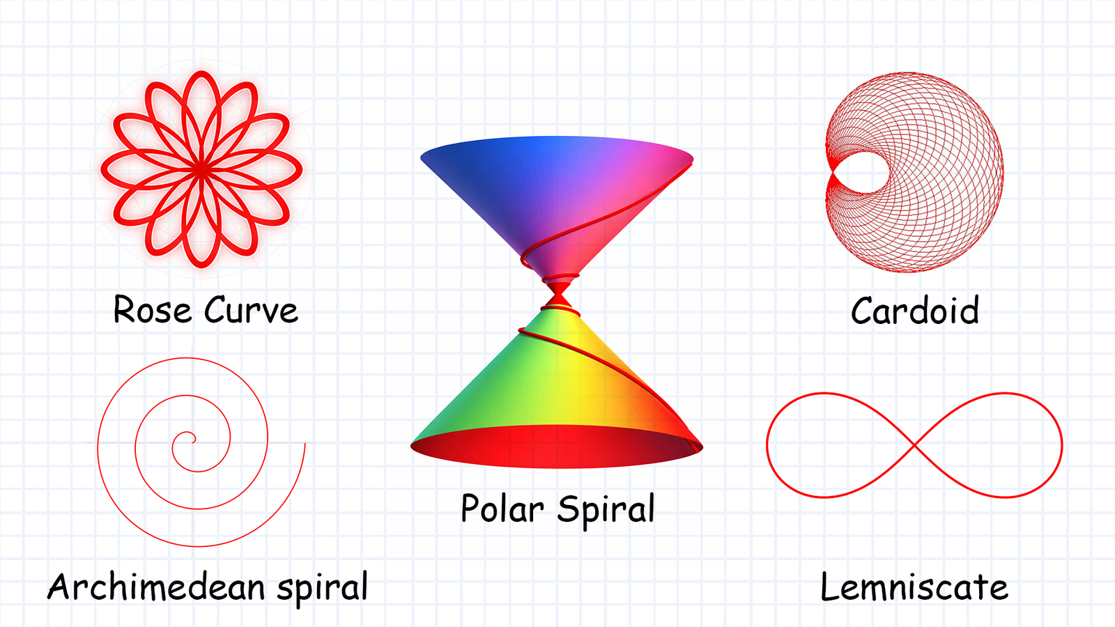
Polar curves are some of the most visually striking objects in mathematics. By expressing relationships in terms of distance and angle rather than horizontal and vertical position, polar equations can produce shapes that would be incredibly complex to describe in Cartesian coordinates. In this guide, we break down every major type of polar curve, from rose curves and cardioids to spirals and lemniscates.
Rose Curves
Rose curves are defined by equations of the form:
r = a cos(nθ) r = a sin(nθ)
Here, a is a real parameter that controls the amplitude and n is a positive integer that determines the symmetry structure of the figure. These equations generate petal-shaped patterns distributed uniformly around the origin.
The geometric behavior depends directly on the parity of n. If n is odd, the curve has exactly n petals. If n is even, the graph produces 2n petals. This difference arises from the periodicity of the trigonometric functions. The function cos(nθ) repeats its values every 2π divided by n, which means the entire figure is constructed through angular repetitions controlled by that factor.
Each petal corresponds to an angular interval where r is positive. When r takes negative values, the point is reflected with respect to the origin, which contributes to the formation of additional petals in the even case. This property reflects an essential feature of polar coordinates: the sign of r directly influences the geometric orientation.
Rose curves possess precise rotational symmetry. When the figure is rotated by an angle of 2π/n, the graph coincides with itself.
Limacons
The class of limacons is defined by the polar equations:
r = a ± b cos(θ) r = a ± b sin(θ)
In these equations, the term a establishes a constant base radial distance, while the trigonometric term introduces a periodic variation that depends on the angle. As a result, the radius is no longer constant and instead oscillates as θ changes.
When θ moves through the interval from 0 to 2π, the value of r alternates between expansion and contraction, generating a closed curve whose shape depends on the relationship between the parameters a and b. If b is small compared to a, the curve approaches a slightly deformed circle. As the trigonometric contribution increases, the deformation becomes more pronounced and the figure acquires the characteristic shape of the limacon.
The name limacon comes from the French limaçon, meaning snail, in reference to the appearance the curve may take. These curves are also known as Pascal’s limacons, in honor of Étienne Pascal.
Lemniscates
Lemniscates are a type of polar curve characterized by quadratic equations in r. A classical example is:
r² = a² cos(2θ) r² = a² sin(2θ)
Here, a is a positive real parameter that determines the scale of the figure. Unlike the curves studied previously, the radial variable appears squared, which introduces an additional symmetry in the structure.
The presence of the term 2θ indicates that the curve is governed by a double angle. This angular duplication introduces strong symmetry in the graph and produces a figure shaped like an infinity symbol composed of two symmetric lobes that meet at the origin. When the equation is r² = a² cos(2θ), the lobes are aligned horizontally with respect to the polar axis. In contrast, when the equation is r² = a² sin(2θ), the figure is rotated so that the lobes are oriented diagonally.
In both cases, the curve is only defined when the trigonometric function is greater than or equal to zero, since r² cannot be negative. This restricts the angular intervals in which real points of the graph exist and determines the regions of the polar plane where each lobe of the lemniscate appears.
When cos(2θ) or sin(2θ) change sign, the equation no longer produces real values of r. This causes the curve to exist only within certain angular intervals and to split into two separate regions. Each lobe corresponds to a distinct interval where the trigonometric function is nonnegative. This angular alternation is what gives rise to the characteristic shape of the lemniscate.
From a geometric point of view, the lemniscate can be interpreted as a polar deformation of a conic, although its structure does not strictly belong to the group of ellipses or hyperbolas. Its central symmetry and its intersection at the origin make it an elegant example of how polar equations can generate curves with deep algebraic and geometric properties.
Cardioids
The cardioid is a particular case of the limacon and is defined by the equations:
r = a(1 ± cos θ) r = a(1 ± sin θ)
Here, a is a positive real parameter that determines the scale of the curve. Its name comes from its resemblance to the shape of a heart.
The distinctive feature of the cardioid is the presence of a cusp at the origin. This appears because r becomes zero when θ = π, which causes the curve to pass exactly through the pole with tangency. Unlike limacons with an inner loop, here there are no negative values of r that generate additional self-intersections.
The symmetry of the curve derives from the cosine function, which implies symmetry with respect to the horizontal axis. If cos θ were replaced by sin θ, the cardioid would be oriented vertically, preserving the same structure but rotated ninety degrees.
From a geometric point of view, the cardioid can be interpreted as the envelope of a family of congruent circles that rotate around another fixed circle. An envelope is the curve that is tangent to each member of a family of curves at some point. This interpretation connects the polar equation with a dynamic process of geometric construction.
The cardioid shows how a linear trigonometric variation in r can produce a curve with a structural singularity, that is, a point where the derivative ceases to behave regularly.
Spirals
Spirals constitute one of the clearest manifestations of the dynamic nature of polar coordinates. Unlike the previous curves, where r oscillates within bounded limits, in spirals the distance from the origin changes steadily as θ increases.
Archimedean Spiral
The Archimedean spiral is defined by:
r = aθ
Here, a is a positive constant that controls the separation between the turns. In this equation, radial growth is linear with respect to the angle. This means that equal increments in θ produce equal increments in r. As a consequence, successive turns remain at a constant distance from each other. The curve neither approaches the origin nor moves away dramatically; its expansion is uniform.
Logarithmic Spiral
The logarithmic spiral satisfies an equation of the form:
r = ae^(bθ)
Here, b is a real constant and the growth is exponential. Each angular increment multiplies the radial distance by a constant factor. This property implies that the shape of the spiral is self-similar, meaning that when the figure is enlarged or reduced, its structure remains invariant. Self-similarity is a geometric property in which a figure preserves its shape under changes of scale.
Hyperbolic Spiral
The hyperbolic spiral is defined by:
r = a/θ
Here, a is a positive constant. In this case the radial behavior is inverse to the angle: as θ increases, the distance from the origin decreases. The curve progressively approaches the pole without reaching it, generating a trajectory that rotates indefinitely while moving closer and closer to the center. This behavior contrasts with growth spirals, since here the angular motion produces radial contraction rather than expansion.
Spirals show that in polar coordinates the angle can act as a variable that generates continuous motion, transforming a simple equation into a trajectory that never closes and extends indefinitely.
Circles
The circle has a particularly simple representation in polar coordinates when it is centered at the origin. The equation:
r = a
Here, a is a positive constant that describes all points whose distance from the origin is exactly a. In this case, θ can take any real value, since the radius remains fixed while the angle moves through the entire interval from 0 to 2π. The resulting curve is a circle of radius a centered at the pole.
What Are Polar Coordinates?
In the Cartesian system, a point in the plane is described by an ordered pair (x, y), which represents horizontal and vertical displacements with respect to the origin. In contrast, in polar coordinates a point is determined by the pair (r, θ), where r is the distance from the origin and θ is the angle measured from the positive horizontal axis.
This system does not decompose motion into perpendicular directions, but rather into magnitude and direction. The radial variable r indicates how far the point is from the pole, while the angle θ specifies its orientation.
A distinctive feature of the polar system is that the same point can have multiple representations. For example, increasing θ by 2π produces the same point, and a negative value of r is equivalent to reflecting the point with respect to the origin while adjusting the angle by π.
Polar coordinates are especially natural when the symmetry of a figure depends on rotations or on distances from the origin. In such cases, the geometric structure is expressed more clearly than in the Cartesian framework.
Conversion Between Cartesian and Polar Coordinates
The relationship between the two systems is given by:
x = r cos θ y = r sin θ
And by the identity:
r² = x² + y²
These expressions allow any equation to be translated from one geometric language to another. For example, the Cartesian circle x² + y² = a² converts directly into r = a.
The conversion between systems is a change of geometric perspective. Some figures are described with extreme simplicity in polar coordinates but become algebraically complex in the Cartesian plane, while others exhibit the opposite behavior.
Leave a Reply